Computationally understanding Einstein's field equation in 1 hour.

This post is trying to explain how to unwrap the Einstein’s field equation into simple differential equations. When I studied general relativity, I spent quite some time in the geometrical structures instead of the physical signification, and I want to summarize the mathematical details here in the bottom-up way.

So when you open Wikipedia and clicked into the page of General Relativity , the first equation you will encounter is the Einstein’s field equations:

\[G_{\mu\nu} \equiv R_{\mu\nu}-\frac{1}{2}R g_{\mu\nu}=\frac{8\pi G}{c^4}T_{\mu\nu}\]

If you have the same background knowledge as I did, then probably you immediately recognize the \(G\) and \(c\) constants, but wtf are the other symbols with subscripts? And if you open an orthodox GR textbook, you will probably revisit the equation in 8+ chapters, if you still haven’t gotten lost in the first 7 chapters.

Well, totally understandable.

Having gone through all the obstacles(probably not entirely useless) and struggled with all the mathematical details, I want to take down these when I still remember them, at least as a refresher in the future.

From scalars to tensors

So it’s obvious, we need to know how \(R_{\mu \nu}\), \(g_{\mu \nu}\) and \(T_{\mu \nu}\) looks like. \(R\) in the equation may seem familiar, but it is actually a scalar variable derived from the \(R_{\mu \nu}\) instead of radius. In summary, we need to know how to represent the three “monsters”.

Let’s talk about their variations from a scalar function, step by step. Firstly, what the \(\mu \nu\) represent? They are just indices from\(\{0 1 2 3\}\), where 0 represent the “time” component, and 1 to 3 is the “space component”. The slightest variation from a scalar function is a vector function, say \(U_{\mu}\), which is the four-velocity of a particle. It is worth knowing that the two variables follow Einstein’s notation, and when you see two identical indices(presumably one lower, one upper as explained next), they represent the summation of all the four possible cases.

Next, The lower and upper location. This is why it is called a (0-2) tensor, instead of just a matrix: The minimum amount of rules you need to know includes that,

1. In GR, the symbols appearing in the super-scripts(sub-scripts) should match exactly those on the other side of the equation, expressions with different structures cannot be equal(0 can be any structure).

2. Symbol with a super-script behaves like the coordinate function, like \(x^{\mu}\). That with a lower-script is a one-form. (No need to shift your focus to it if you haven’t learnt it.).

3. If you need to move a symbol downward, you need to multiply the tensor by the metric tensor \(g_{\mu\, \nu}\), that is, \(F^{\mu}_{\gamma} g_{\mu \nu}=F_{\nu \gamma}\). (The sequence matters, but we will ignore it here.)

4. (Optional) You can contract a tensor by having another tensor with symbol in the other-script. Such as, \(T_{\mu\nu}U^{\mu}V^{\nu}\) is the inner product of the T-matrix with the two column vectors.

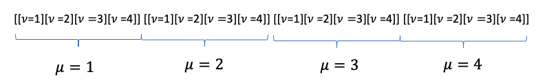
To visualize the tensor(say the (0-2) case), you can somewhat understand it as a bundle of 16 scalar functions. It can be seen as picking the corresponding \(\mu\, \nu\) in the row vector shown below sequentially, and also in the corresponding \(U^{\mu}V^{\nu}\) column vector, and add up all variations. From this we can see why the super/sub-script matters.

Structure of (0-2) tensor

The metric and the stress-energy tensor

Before getting into the pure mathematical definition, let’s get a little knowledge about the two symbols \(g_{\mu \nu}\) and \(T_{\mu \nu}\).

\(g_{\mu \nu}\), the metric tensor, describes the metric-defined distance between the two points, and more importantly serves as the bridge between lower-index and upper-index. From special relativity, we know that the proper length is

\[\Delta S= \Delta x^2+ \Delta y^2 + \Delta z^2 - c^2 \Delta t^2,\]

which can be understood as the inner product between the four vectors \(\Delta x^{\mu}\) and the Minkowski metric:

\[\eta= \begin{bmatrix} -c^2 & 0 & 0 & 0\\ 0 & 1 & 0 & 0\\ 0 & 0 & 1 & 0\\ 0& 0& 1 & 1 \end{bmatrix}\]

(It should be made clear that even though the metric is commonly represented as matrix, their structures are different: More rigorous structure is shown above, but we will just use the matrix representation.)

Again, in the simplest language, the metric tensor is a 16-component vector with individual scalar function depending on the 4-vector, and it reflects the local structure of spacetime.

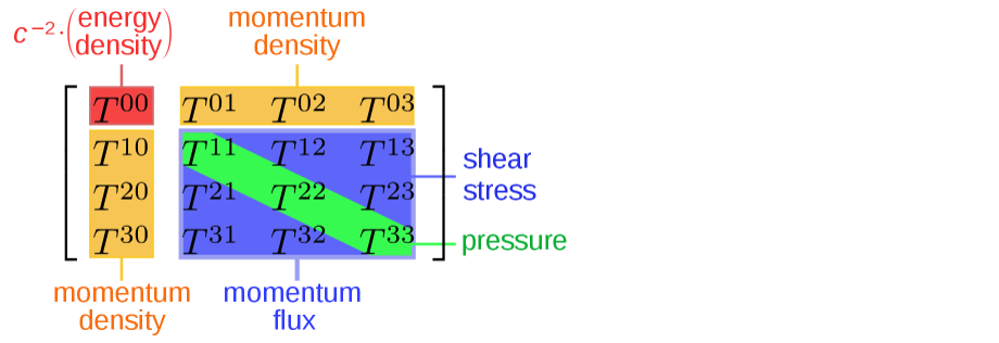
The stress-energy tensor, \(T_{\mu \nu}\), reflects the local energy density and energy flux.

The time–time component is the density of relativistic mass, i.e., the energy density divided by the speed of light squared. The flux of relativistic mass across the \(x^k\) surface is equivalent to the density of the k-th component of linear momentum, i.e., the momentum density in the figure; the components \(T^{kl}\) represent flux of k-th component of linear momentum across the \(x^l\) surface. (The whole paragraph is copied from Wikipedia.)

Structure of stress-energy tensor

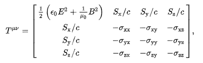
One example is the case where there is only EM field in space, and then the SE tensor can be represented from the energy density, the Poynting vector and the Maxwell stress tensor:

Electromagnetic SE tensor

Covariant derivatives

So now we can interpret that the RHS of Einstein’s equation, the energy density and flux, can influence(and be influenced by) the spacetime structure. However, we can see immediately that if we ignore the term \(R_{\mu\nu}\), then the line is a zero-order linear equation, which doesn’t make sense as the spacetime is not propagating, so the first term must involve derivatives, and that’s what we are going to discuss next.

I will bring up the final form first: the term \(R_{\mu\nu}\) is a function of the second derivatives of the metric tensor. Again, we will mainly focus on the tensor structure instead of physical interpretation.

First we introduce the covariant derivative, the counterpart in changing coordinate systems: we know that in polar coordinates the derivative

\[\frac{\partial \vec{V}}{\partial r} =\frac{\partial \vec{V}^{\alpha}}{\partial r} {\vec{e}_{\alpha}} + V^{\alpha}\frac{\partial \vec{V}_{\alpha}}{\partial r}\]

Covariant and directional derivative

(Cited from here ).

where the second term comes from the rotating coordinate system, and it is similar in general relativity, where the spacetime is curved: We introduce the Christoffel symbol, whose definition is

\[\frac{\partial \vec{e}_{\alpha}}{\partial x^{\beta}} = {\Gamma^{\mu}}_{\alpha\beta} \vec{e}_{\mu}.\]

We can see clearly that the second term calculates the connection between the global and the basis vector. Going back to our discussion, the component-form Christoffel symbol is

\[{\Gamma^{\alpha}}_{\mu\nu} = \frac{1}{2} g^{\alpha\beta} (g_{\beta \mu,\nu}+g_{\beta \nu,\mu}-g_{\mu\nu,\beta})\]

The comma means the local derivative. So it’s obvious here that the Christoffel symbol is a (1-2) tensor which involves the zero- and first-order derivatives of the metric tensor.

Reimann curvature and Ricci tensor.

Congratulations you have reached so far! Now is the final step before we recover the whole field equation. You may have noticed that what we want eventually is a (0-2) tensor, so there are some further manipulations. Firstly, we introduce the Riemann tensor, which is defined as

\[{R^{\alpha}}_{\beta\mu\nu} = {\Gamma^{\alpha}}_{\beta \nu,\mu} - {\Gamma^{\alpha}}_{\beta \mu,\nu} + {\Gamma^{\alpha}}_{\sigma\mu} {\Gamma^{\alpha}}_{\beta\nu} - {\Gamma^{\alpha}}_{\sigma\nu} {\Gamma^{\alpha}}_{\beta\mu}.\]

This term comes from taking a closed loop and calculating the change in the vector due to transport. A more straightforward representation is

\[{R^{\alpha}}_{\beta\mu\nu} = \frac{1}{2} G^{\sigma \sigma} (g_{\sigma \nu,\beta \mu} - g_{\sigma \mu,\beta \nu} +g_{\beta \mu,\sigma \nu} -g_{\beta \nu,\sigma \mu}).\]

Then we contract the Riemann tensor, and get Ricci tensor:

\[R_{\alpha \beta} = {R^{\mu}}_{\sigma\mu\beta}\]

and the Ricci scalar

\[R = g^{\mu \nu} R_{\mu \nu} = g^{\mu \nu} g^{\alpha \beta} R_{\alpha \mu \beta \nu}.\]

If you still remember the field equation, you can see that these are the (0-2) R tensor and R scalar in it, so we can conclude the structure of Einstein field equation right now: the LHS is 16-component functions of the metric tensor and the second derivative of it, which describes the local geometric deformation, and the RHS is the 16-component function of the stress energy tensor. That’s it!